ANALYSIS OF ALGORITHM

Unit I — Elementary Algorithmic & Asymptotic Notation:

The Efficiency of Algorithms, Average and Worst-Case Analyses, Amortized Analysis, A Notation For “The Order Of”, Asymptotic Notations: Conditional, With Parameters, Operations: Asymptotic Notation.

Efficiency of Algorithms

A good algorithm is correct, but a great algorithm is both correct and efficient. The most efficient algorithm is one that takes the least amount of execution time and memory usage possible while still yielding a correct answer.

Performance

Two areas are important for performance:

1. space efficiency — the memory required, also called, space complexity
2. time efficiency — the time required, also called time complexity

Space Efficiency

There are some circumstances where the space/memory used must be analyzed. For example, for large quantities of data or for embedded systems programming.

Components of space/memory use:

1. instruction spaceAffected by: the compiler, compiler options, target computer (cpu)2. data spaceAffected by: the data size/dynamically allocated memory, static program variables,3. run-time stack spaceAffected by: the compiler, run-time function calls and recursion, local variables, parameters

The space requirement has fixed/static/compile time and a variable/dynamic/runtime components. Fixed components are the machine language instructions and static variables. Variable components are the runtime stack usage and dynamically allocated memory usage.

One circumstance to be aware of is, does the approach require the data to be duplicated in memory (as does merge sort). If so we have 2N memory use.

Space efficiency is something we will try to maintain a general awareness of.

Time Efficiency

Clearly the more quickly a program/function accomplishes its task the better.

The actual running time depends on many factors:

• The speed of the computer: cpu (not just clock speed), I/O, etc.
• The compiler, compiler options .
• The quantity of data — ex. search a long list or short.
• The actual data — ex. in the sequential search if the name is first or last.

Time Efficiency — Approaches

When analyzing for time complexity we can take two approaches:

1. Order of magnitude/asymptotic categorization — This uses coarse categories and gives a general idea of performance. If algorithms fall into the same category, if data size is small, or if performance is critical, then the next approach can be looked at more closely.
2. Estimation of running time -
   By analysis of the code we can do:
3. operation counts — select operation(s) that are executed most frequently and determine how many times each is done.
4. step counts — determine the total number of steps, possibly lines of code, executed by the program.
5. By execution of the code we can:
6. benchmark — run the program on various data sets and measure the performance.
7. profile — A report on the amounts of time spent in each routine of a program, used to find and tune away the hot spots in it. This sense is often verbed. Some profiling modes report units other than time (such as call counts) and/or report at granularities other than per-routine, but the idea is similar (from foldoc).
   Look at the info entry for gprof on one of the linux machines.

Time Efficiency — Three Cases

For any time complexity consideration there are 3 cases:

1. worst case
2. average case
3. best case

Usually worst case is considered since it gives an upper bound on the performance that can be expected. Additionally, the average case is usually harder to determine (its usually more data dependent), and is often the same as the worst case. Under some circumstances it may be necessary to analyze all 3 cases (algorithms topic).

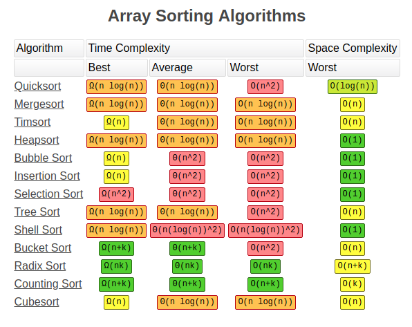
Algorithmic Common Runtimes

The common algorithmic runtimes from fastest to slowest are:

• constant: Θ(1)
• logarithmic: Θ(log N)
• linear: Θ(N)
• polynomial: Θ(N²)
• exponential: Θ(2^N)
• factorial: Θ(N!)

EXAMPLE

algorithm efficiency A measure of the average execution time necessary for an algorithm to complete work on a set of data. Algorithm efficiency is characterized by its order. Typically a bubble sort algorithm will have efficiency in sorting N items proportional to and of the order of N2, usually written O(N2). This is because an average of N/2 comparisons are required N/2 times, giving N2/4 total comparisons, hence of the order of N2. In contrast, quicksort has an efficiency O(N log2N).

If two algorithms for the same problem are of the same order then they are approximately as efficient in terms of computation. Algorithm efficiency is useful for quantifying the implementation difficulties of certain problems.